Neural Motifs: Scene Graph Parsing with Global Context
last modified : 05-09-2018
General Information
- Title: Neural Motifs: Scene Graph Parsing with Global Context
- Authors: Rowan Zellers, Mark Yatskar, Sam Thomson, Yejin Choi, Paul G. Allen
- Link: article
- Date of first submission: 17 november 2017
- Implementations:
Brief
This article builds a network that uses both local and global structure. Their architecture is justified by a statistical analysis of the graphs used.
They show that some objects in the dataset are strongly linked to some other and that if you have the two objects there is a high probability to get some relation between the objects.
How Does It Work
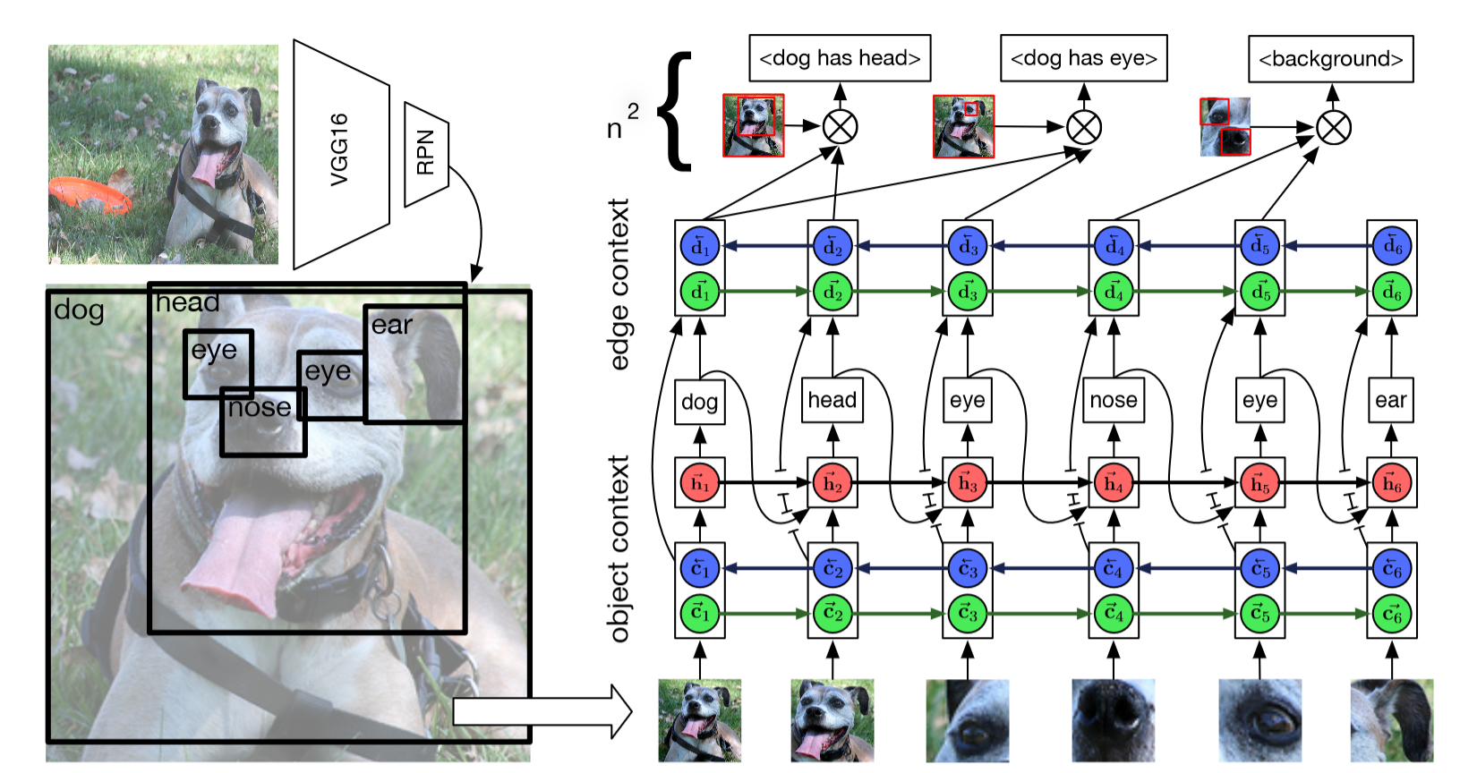
Their structure is made a series of lstm layers to take advantage of the global structure of the graph while at the same time still having the local information.
The following figure shows the pipeline for creating a graph from an image:

The relation between the dog and the eye is kept thanks to the lstm.
Results
For the results, SGD stands for Scene Graph Detection, SGC for Scene Graph Classification and PC for Predicate Classification.
The Freq and Freq + overlap are association for the relation using the frequencies extracted from the dataset. The overlap means that the non overlapping object were set as BackGround.
The motifnet are the networks developed in the article:
- Motifnet leftright: The boxes were parsed from left to right
- Motifnet nocontext: The context part was remove from the network
- Motifnet Confidence: The order of the parsing of the boxes is made by confidence
- Motifnet Size: The order of the parsing of the boxes is from biggest to smallest
- Motifnet Random: The order of the parsing of the boxes is random
| | SGD | SGD | SGD | SGC | SGC | SGC | PC | PC | PC | Mean `| |:-:|:-:|:-:|:-:|:-:|:-:|:-:|:-:|:-:|:-:|:-:|:-:| Model | R@20 | R@50 | R@100 | R@20 | R@50 | R@100 | R@20 | R@50 | R@ 100 | | VRD | | 0.3 | 0.5 | | 11.8 | 14.1 | | 27.9 | 35.0 | 14.9 | | MESSAGEPASSING | | 3.4 | 4.2 | | 21.7 | 24.4 | | 44.8 | 53.0 | 25.3 | | MESSAGEPASSING+ | 14.6 | 20.7 | 24.5 | 31.7 | 34.6 | 35.4 | 52.7 | 59.3 | 61.3 | 39.3 | | ASSOCEMBED | 6.5 | 8.1 | 8.2 | 18.2 | 21.8 | 22.6 | 47.9 | 54.1 | 55.4 | 28.3 | | FREQ | 17.7 | 23.5 | 27.6 | 27.7 | 32.4 | 34.0 | 49.4 | 59.9 | 64.1 | 40.2 | | FREQ+OVERLAP | 20.1 | 26.2 | 30.1 | 29.3 | 32.3 | 32.9 | 53.6 | 60.6 | 62.2 | 40.7 | | MOTIFNET-LEFTRIGHT | 21.4 | 27.2 | 30.3 | 32.9 | 35.8 | 36.5 | 58.5 | 65.2 | 67.1 | 43.6 | | MOTIFNET-NOCONTEXT | 21.0 | 26.2 | 29.0 | 31.9 | 34.8 | 35.5 | 57.0 | 63.7 | 65.6 | 42.4 | | MOTIFNET-CONFIDENCE | 21.7 | 27.3 | 30.5 | 32.6 | 35.4 | 36.1 | 58.2 | 65.1 | 67.0 | 43.5 | MOTIFNET-SIZE | 21.6 | 27.3 | 30.4 | 32.2 | 35.0 | 35.7 | 58.0 | 64.9 | 66.8 | 43.3 | | MOTIFNET-RANDOM | 21.6 | 27.3 | 30.4 | 32.5 | 35.5 | 36.2 | 58.1 | 65.1 | 66.9 | 43.5 |
In Depth
The network has several steps, all shown in the figure below :

First the potential object in the image are extracted using a usual classifier (faster R-CNN here). Then context is extracted from each of the potential objects, this steps uses bilateral LSTM to take into account the potential relation between the objects. After that a LSTM is used to extract the boxes classes. Finally edge context is extracted using again bidirectional LSTM and the probality for the edges label are then computed for each possible relation between object, that is .