Deformable Convolutional Networks
last modified : 27-11-2018
General Information
- Title: Deformable Convolutional Networks
- Authors: Jifeng Dai, Haozhi Qi, yYuwen Xiong, Yi Li, Guodong Zhang, Han Hu, Yichen Wei
- Link: article
- Date of first submission: 17 March 2017
- Implementations:
Brief
In this paper, the authors argue that neural networks are limited to model geometric transformation due to the fixed nature of the layers making up the network. To remove this constraint, they introduce layers that can adapt to the shape of the object to locate (i.e rather than forcing the network into some pre-set filters, let it learn for itself what is best). The deformable layers can replace any layers in any network easily with not much increase in the computation cost (deformable convolutional layers can replace convolutional layers, deformable pooling layers can replace pooling layer). Their layers can be learnt through back-propagation.
How Does It Work
The articles presents 3 types of layers, the deformable convolution, the deformable RoI pooling and the deformable PS RoI pooling.
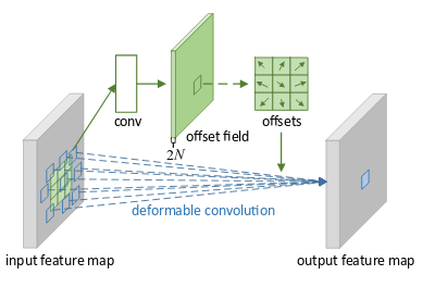
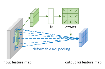
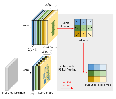
All the deformable layers are fairly similar in conception, a branch process the input feature map to get the offsets, and then bilinear interpolation is applied to the input feature map at the position of the offset to get the value of the output.
Deformable Convolution:

Deformable roi pooling:

Deformable ps roi pooling:

Results
The table below shows the results of various architecture with and without the deformable layers. The architecture with the deformable layers performs systematically better than the ones without.
Object detection results of deformable ConvNets v.s. plain ConvNets on COCO test-dev set. M denotes multi-scale testing, and B denotes iterative bounding box average:
| method | backbone architecture | M | B | mAP@(0.5:0.95) | mAP@0.5 | mAP@(0.5:0.95) (small) | mAP@(0.5:0.95) (mid) | mAP@(0.5:0.95) (large) |
|---|---|---|---|---|---|---|---|---|
| class-aware RPN | ResNet-101 | 23.2 | 42.6 | 6.9 | 27.1 | 35.1 | ||
| Ours | ResNet-101 | 25.8 | 45.9 | 7.2 | 28.3 | 40. 7 | ||
| Faster RCNN | ResNet-101 | 29.4 | 48.0 | 9.0 | 30.5 | 47.1 | ||
| Ours | ResNet-101 | 33.1 | 50.3 | 11.6 | 34.9 | 51. 2 | ||
| R-FCN | ResNet-101 | 30.8 | 52.6 | 11.8 | 33.9 | 44.8 | ||
| Ours | ResNet-101 | 34.5 | 55.0 | 14.0 | 37.7 | 50. 3 | ||
| Faster RCNN | Aligned-Inception-ResNet | 30.8 | 49.6 | 9.6 | 32.5 | 49.0 | ||
| Ours | Aligned-Inception-ResNet | 34.1 | 51.1 | 12.2 | 36.5 | 52.4 | ||
| R-FCN | Aligned-Inception-ResNet | 32.9 | 54.5 | 12.5 | 36.3 | 48.3 | ||
| Ours | Aligned-Inception-ResNet | 36.1 | 56.7 | 14.8 | 39.8 | 52.2 | ||
| R-FCN | Aligned-Inception-ResNet | X | 34.5 | 55.0 | 16.8 | 37.3 | 48.3 | |
| Ours | Aligned-Inception-ResNet | X | 37.1 | 57.3 | 18.8 | 39.7 | 52.3 | |
| R-FCN | Aligned-Inception-ResNet | X | X | 35.5 | 55.6 | 17.8 | 38.4 | 49.3 |
| Ours | Aligned-Inception-ResNet | X | X | 37.5 | 58.0 | 19.4 | 40.1 | 52.5 |
In Depth
Deformable Convolution

A convolution is applied to the input feature map. The offset field is of size 2N (N 2D offset, [(x1,y1), (x2, y2), ...]). Then for a position on the output map, the value is calculated using the offsets.
The input and output feature maps have the same dimension and if the offset is in between cells in the grid, the values for the convolution are interpolated.
The conv layer is learned with backpropagation.
The other layers work in a similar fashion, see the article for more details on the other layers.