SSD

last modified : 13-06-2019

General Information

• Title: SSD: Single Shot MultiBox Detector
• Authors: Wei Liu, Dragomir Anguelov, Dumitru Erhan, Christian Szegedy, Scott Reed
• Link: article
• Date of first submission: 8 Dec 2015
• Implementations:
  • Keras
  • Caffe

Brief

The SSD is a one-shot detector in the same style as the YOLO. The main advantage of this network is to be fast with a pretty good accuracy. When it was published its scoring was among the best in the PASCAL VOC challenge regarding both the mAP (72.1% mAP) and the number of fps (58) (using a Nvidia Titan X), beating its main concurrent at the time, the YOLO (which has since be improved).

How Does It Work

Even if it is a one shot detector, the network can be divided into two parts, a feature extractor, the VGG16, and regressors/classifiers using convolutional layers at different scales. The novel idea is to downsize the feature map output by the VGG16 using convolution and pooling layers to get the different scales.

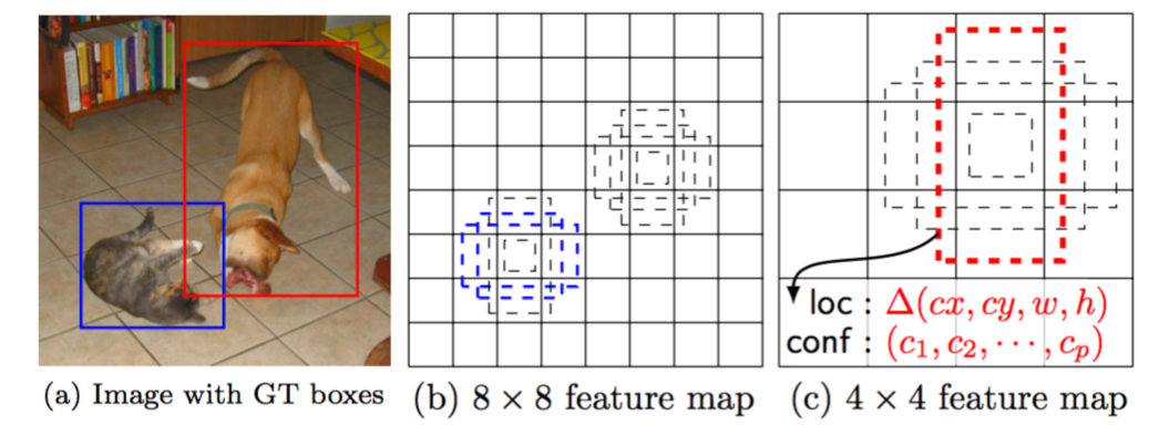
Then, the network uses grids of various scale to predict the different boxes present in the image. The SSD outputs pre-defined sets boxes for different grids and tells for each box if there is (or isn't) an object in each box.

The following image, taken from the original paper, shows two grid and the matching between objects and pre-set boxes:

There are two grids shown, for each of those grids there is a number of pre-set boxes that can match the ground truth boxes (only a few are on the diagrams). The network tells for each box if it matches or not an object in the image (here two matches for the cat and one for the dog). The bigger the grid, the smaller the object detected is, this is how the SSD allows for multiple detections in one shot. It is also to be noted that the boxes coordinates are regressed to add in precision.

Results

• PASCAL VOC 2007:

Method	data	mAP
SSD300	07	68.0
SSD300	07+12	74.3
SSD300	07+12+COCO	79.6
SSD512	07	71.6
SSD512	07+12	76.8
SSD512	07+12+COCO	81.6

• PASCAL VOC 2012:

Method	data	mAP
SSD300	07++12	72.4
SSD300	07++12+COCO	77.5
SSD512	07++12	74.9
SSD512	07++12+COCO	80.0

In Depth

Architecture

The SSD can be divided into two main parts, the feature extractor and the regressors/classifiers. For the first part, the VGG-16 is used, then convolutional layers are added to create the grids used for the classifications/predictions. The image below shows the architecture of the network :

As can be seen the network outputs 8732 boxes, we can separate the boxes in 6 groups, one per scale for the boxes inferred. Each group is supposed to detect different size objects, the closer we are from the VGG-16 the smaller the object.

For each group of boxes, the numbers are as follows:

• from conv4_3, 5776 boxes for a detection size around 0.1 of the original image size
• from conv7, 2166 boxes for a detection size around 0.2 of the original image size
• from conv8_2, 600 boxes for a detection size around 0.38 of the original image size
• from conv9_2, 150 boxes for a detection size around 0.56 of the original image size
• from conv10_2, 36 boxes for a detection size around 0.74 of the original image size
• from conv11_2, 4 boxes for a detection size around 0.92 of the original image size

To explain a bit the numbers in the diagram and how using convolution one can go from filter map to boxes, let's take an example: the boxes obtained from the layer conv_9_2.

The grid is 5x5, for a total of 25 cells. For each cell 6 boxes will be predicted using a 3x3 convolution, so we have 3x3x(64) (4 for the coordinates of the box). In addition to that, for each box, we need to tell the class associated, thus we have 3x3x(6 *(Classes+4)).

Loss

The loss function used for the network is the following one:

$$L(x,c,l,g) = \frac{1}{N} (L_{conf}(x,c) + \alpha L_{loc}(x,l,g))$$

With x being an indicator for matching default and ground truth box, c the confidences, l the predicted boxes, g the ground truth boxes. For more detail on the function, please refer to the original article.

The important part is the modification of the loss function to fit the huge number of boxes. All the boxes are either matched to an object or to the background. Because of this matching strategy, there is a lot more of unmatched box than matched box. This creates an imbalance for the training which could get the network to predict all the boxes as background. That is why the loss function uses a maximum ratio between the matched and unmatched boxes. Basically, the Lconf and Lloc are not over all the boxes but a few of them.

To be Noted

An important unspecified point, in the paper the bounding boxes are regressed, but in the implementation they are also divided by some term that is here to account as some kind of variance. One could see this as some normalization to take into account the differences a person who would tag the data would make if he/she was to be tagging two times the same image.